Master Compression and Clipping Analysis
In this post I want to analyze clipping/ limiting and compression by looking at songs that are plotted as a histogram of the normalized amplitudes of the song waveform. Normalized meaning the maximum song waveform value is 1 and the minimum is -1.
The x-axis is the amplitude of the audio signal and the y-axis is the density of samples at that amplitude.
Terms:
RMS: Root Mean Square. The square root of the mean of the squared amplitudes. It represents the power of the song. σ = √[(1/N) × Σ(x²)] It is the same calculation as the standard deviation with audio having roughly a 0 mean.
Crest Factor: The ratio of the peak amplitude to the RMS amplitude. It measures the dynamic range. Higher values imply less compression and more dynamic range and lower volues imply more compression and less dynamic range.
Relatively Uncompressed and Unclipped
Before we dive in let's look at a song that is relatively uncompressed and unclipped
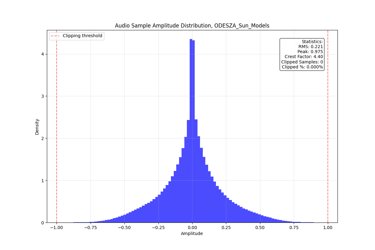
Above is a standard looking song that doesn't appear to have much compression or clipping. Compare this with the images below
Compression and a Little Clipping
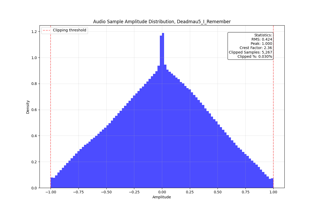
This is a histogram of the deadmau5 song "I Remember". You can see the spikes at the edges of the histogram, which represent clipping. It also moves out linearly like a pyramid, which I believe implies the linear compression ratio being applied beyond the threshold. This makes quiet sounds relatively louder to the peak sounds and when you apply makeup gain it draws the sounds close to zero out toward the edges. This is why this song looks different than the Odesza song.
Compression and Heavy Clipping
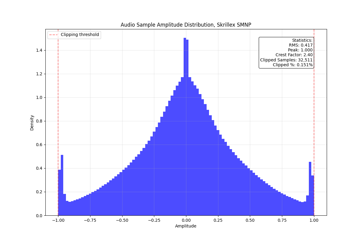
The image above is a histogram of the skrillex song "Scary Monsters and Nice Sprites". Again you can see the spikes at the edges of the histogram. This song is clipping/ saturating a lot for maximum loudness. He is also using a lot of compression which is why the distribution is wider and the crest factor is lower. This crest factor again is the difference between the rms value and the maximum. The closer the rms to the peak means the rms value is further from zero and the quiet parts are louder i.e. further away from zero.